Surrogate Replacement Workflow

This notebook demonstrates the full workflow for replacing a computationally expensive component in a multi-component OpenMDAO assembly with a surrogate model. The workflow uses standard_evaluator to:

1. Build a multi-component assembly with aerodynamics, structures, and performance groups

2. Capture the assembly interface and extract the expensive sub-group

3. Train a polynomial surrogate on the isolated sub-group

4. Replace the expensive component with the surrogate in the assembly description

5. Compare three evaluation approaches: original assembly, locally-replaced assembly, and a global surrogate

All components use ExecComp (no external dependencies), making this notebook fully reproducible. The aerodynamics group uses internal connect() calls to demonstrate proper handling of connection metadata.

import numpy as np
import pandas as pd
import matplotlib.pyplot as plt
import openmdao.api as om
import standard_evaluator as se
from standard_evaluator.evaluators import OpenMDAOEvaluator

matlabengine not available.

1. Creating the Multi-Component Assembly

We build an assembly with three sub-groups:

• aero — Aerodynamics group computing dynamic pressure, lift, and drag. Uses internal connect() to pass the pressure output to lift and drag calculations. Mark the variables and responses that are internal with the ‘internal’ tag.

• structures — Structural analysis computing weight and stress from material/geometry parameters.

• performance — Performance metric combining aero and fuel parameters to compute range.

The top-level assembly uses promotions (promotes=['*']) to connect the groups together.

# Build the assembly
assembly = om.Group()

# --- Aero group (with internal connect) ---
aero = om.Group()
aero.add_subsystem(
    'pressure_calc',
    om.ExecComp('pressure = 0.5 * rho * v**2', pressure={'tags': 'internal'}),
    promotes_inputs=['rho', 'v']
)
aero.add_subsystem(
    'lift_calc',
    om.ExecComp('lift = cl * q * area', q={'tags': 'internal'}),
    promotes_inputs=['cl', 'area'],
    promotes_outputs=['lift']
)
aero.add_subsystem(
    'drag_calc',
    om.ExecComp('drag = cd * q * area', q={'tags': 'internal'}),
    promotes_inputs=['cd', 'area'],
    promotes_outputs=['drag']
)
# Internal connections: pressure output feeds lift and drag calculations
aero.connect('pressure_calc.pressure', 'lift_calc.q')
aero.connect('pressure_calc.pressure', 'drag_calc.q')

# --- Structures group ---
structures = om.Group()
structures.add_subsystem(
    'weight_calc',
    om.ExecComp('weight = density * volume * 9.81'),
    promotes_inputs=['density', 'volume'],
    promotes_outputs=['weight']
)
structures.add_subsystem(
    'stress_calc',
    om.ExecComp('stress = force / area_struct'),
    promotes_inputs=['force', 'area_struct'],
    promotes_outputs=['stress']
)

# --- Performance group ---
performance = om.Group()
performance.add_subsystem(
    'range_calc',
    om.ExecComp('range_out = (lift / drag) * (fuel / sfc)'),
    promotes_inputs=['lift', 'drag', 'fuel', 'sfc'],
    promotes_outputs=['range_out']
)

# --- Top-level assembly with promotions ---
assembly.add_subsystem('aero', aero, promotes=['*'])
assembly.add_subsystem('structures', structures, promotes=['*'])
assembly.add_subsystem('performance', performance, promotes=['*'])

# Create and setup the problem
prob = om.Problem(model=assembly)
prob.setup()
prob.final_setup()

# Set input values
prob.set_val('rho', 1.225)       # air density [kg/m^3]
prob.set_val('v', 50.0)          # velocity [m/s]
prob.set_val('cl', 0.5)          # lift coefficient
prob.set_val('cd', 0.03)         # drag coefficient
prob.set_val('area', 20.0)       # wing area [m^2]
prob.set_val('density', 2700.0)  # material density [kg/m^3]
prob.set_val('volume', 0.01)     # structural volume [m^3]
prob.set_val('force', 5000.0)    # applied force [N]
prob.set_val('area_struct', 0.005)  # structural cross-section area [m^2]
prob.set_val('fuel', 500.0)      # fuel mass [kg]
prob.set_val('sfc', 0.5)         # specific fuel consumption [1/hr]

prob.run_model()

print('Assembly outputs:')
print(f"  pressure = {prob.get_val('aero.pressure_calc.pressure')[0]:.4f} Pa")
print(f"  lift     = {prob.get_val('lift')[0]:.4f} N")
print(f"  drag     = {prob.get_val('drag')[0]:.4f} N")
print(f"  weight   = {prob.get_val('weight')[0]:.4f} N")
print(f"  stress   = {prob.get_val('stress')[0]:.4f} Pa")
print(f"  range    = {prob.get_val('range_out')[0]:.4f}")

Assembly outputs:
  pressure = 1531.2500 Pa
  lift     = 15312.5000 N
  drag     = 918.7500 N
  weight   = 264.8700 N
  stress   = 1000000.0000 Pa
  range    = 16666.6667

2. Capturing the Interface and Extracting the Aero Sub-Group

With the assembly built and verified, we now use standard_evaluator to:

1. Capture the full assembly interface as a serializable GroupInfo description using se.get_interface()

2. Display the hierarchical structure with se.show_structure() to see all components, inputs, outputs, promotions, and linkages

3. Extract the aerodynamics sub-group from the assembly description and reconstruct it as a standalone OpenMDAO Problem using se.create_problem()

4. Wrap the extracted problem as an OpenMDAOEvaluator so it can be sampled for surrogate training

This demonstrates the key capability of standard_evaluator: converting between live OpenMDAO assemblies and portable interface descriptions that can be inspected, modified, and reconstructed.

Note: If there are connections that are made inside a group that should stay internal it is important to add the internal tag to the inputs or outputs.

We also set bounds for the variables and create an optimization problem that will be used later when exposing the OpenMDAO problem as an evaluator.

# Capture the full assembly interface as a GroupInfo description
assembly_info = se.get_interface(assembly)

se.set_variable_bounds(assembly_info, {
    'rho': (0.5, 2.0), 'v': (10, 100),
    'cl': (0.1, 1.5), 'cd': (0.01, 0.3), 'area': (5, 50),
    'density': (2000, 4000), 'volume': (0.001, 0.5),
    'force': (4000.0, 6000.0), 'area_struct': (0.002, 0.008),
    'fuel': (300.0, 600.0), 'sfc': (0.3, 0.8) })
# Build the se problem with those bounds
full_opt_problem = se.build_opt_problem(assembly_info, prob)

# Display the hierarchical assembly structure
print("Assembly structure:")
print("=" * 60)
se.show_structure(assembly_info)
print(full_opt_problem)

Assembly structure:
============================================================
 1  15 6
 Inputs:  ['area', 'cd', 'drag_calc.q', 'cl', 'lift_calc.q', 'rho', 'v', 'drag', 'fuel', 'lift', 'sfc', 'area_struct', 'force', 'density', 'volume']
 Outputs: ['drag', 'lift', 'pressure_calc.pressure', 'range_out', 'stress', 'weight']
 Promotions: {'aero': [('area', 'area'), ('cd', 'cd'), ('area', 'area'), ('cl', 'cl'), ('rho', 'rho'), ('v', 'v'), ('drag', 'drag'), ('lift', 'lift')], 'structures': [('area_struct', 'area_struct'), ('force', 'force'), ('density', 'density'), ('volume', 'volume'), ('stress', 'stress'), ('weight', 'weight')], 'performance': [('drag', 'drag'), ('fuel', 'fuel'), ('lift', 'lift'), ('sfc', 'sfc'), ('range_out', 'range_out')]}
 Linkage   : []
   2 aero 7 3
   Inputs:  ['area', 'cd', 'drag_calc.q', 'cl', 'lift_calc.q', 'rho', 'v']
   Outputs: ['drag', 'lift', 'pressure_calc.pressure']
   Promotions: {'pressure_calc': [('rho', 'rho'), ('v', 'v')], 'lift_calc': [('area', 'area'), ('cl', 'cl'), ('lift', 'lift')], 'drag_calc': [('area', 'area'), ('cd', 'cd'), ('drag', 'drag')]}
   Linkage   : [('pressure_calc.pressure', 'lift_calc.q'), ('pressure_calc.pressure', 'drag_calc.q')]
     3 pressure_calc 2 1
     Inputs:  ['rho', 'v']
     Outputs: ['pressure']
     4 lift_calc 3 1
     Inputs:  ['area', 'cl', 'q']
     Outputs: ['lift']
     5 drag_calc 3 1
     Inputs:  ['area', 'cd', 'q']
     Outputs: ['drag']
   6 structures 4 2
   Inputs:  ['area_struct', 'force', 'density', 'volume']
   Outputs: ['stress', 'weight']
   Promotions: {'weight_calc': [('density', 'density'), ('volume', 'volume'), ('weight', 'weight')], 'stress_calc': [('area_struct', 'area_struct'), ('force', 'force'), ('stress', 'stress')]}
   Linkage   : []
     7 weight_calc 2 1
     Inputs:  ['density', 'volume']
     Outputs: ['weight']
     8 stress_calc 2 1
     Inputs:  ['area_struct', 'force']
     Outputs: ['stress']
   9 performance 4 1
   Inputs:  ['drag', 'fuel', 'lift', 'sfc']
   Outputs: ['range_out']
   Promotions: {'range_calc': [('drag', 'drag'), ('fuel', 'fuel'), ('lift', 'lift'), ('sfc', 'sfc'), ('range_out', 'range_out')]}
   Linkage   : []
     10 range_calc 4 1
     Inputs:  ['drag', 'fuel', 'lift', 'sfc']
     Outputs: ['range_out']
name='from_interface' class_type='OptProblem' variables=[FloatVariable(name='area', default=None, bounds=(5.0, 50.0), shift=0.0, scale=1.0, units=None, description='', options={}, class_type='float'), FloatVariable(name='cd', default=None, bounds=(0.01, 0.3), shift=0.0, scale=1.0, units=None, description='', options={}, class_type='float'), FloatVariable(name='cl', default=None, bounds=(0.1, 1.5), shift=0.0, scale=1.0, units=None, description='', options={}, class_type='float'), FloatVariable(name='rho', default=None, bounds=(0.5, 2.0), shift=0.0, scale=1.0, units=None, description='', options={}, class_type='float'), FloatVariable(name='v', default=None, bounds=(10.0, 100.0), shift=0.0, scale=1.0, units=None, description='', options={}, class_type='float'), FloatVariable(name='fuel', default=None, bounds=(300.0, 600.0), shift=0.0, scale=1.0, units=None, description='', options={}, class_type='float'), FloatVariable(name='sfc', default=None, bounds=(0.3, 0.8), shift=0.0, scale=1.0, units=None, description='', options={}, class_type='float'), FloatVariable(name='area_struct', default=None, bounds=(0.002, 0.008), shift=0.0, scale=1.0, units=None, description='', options={}, class_type='float'), FloatVariable(name='force', default=None, bounds=(4000.0, 6000.0), shift=0.0, scale=1.0, units=None, description='', options={}, class_type='float'), FloatVariable(name='density', default=None, bounds=(2000.0, 4000.0), shift=0.0, scale=1.0, units=None, description='', options={}, class_type='float'), FloatVariable(name='volume', default=None, bounds=(0.001, 0.5), shift=0.0, scale=1.0, units=None, description='', options={}, class_type='float')] responses=[FloatVariable(name='drag', default=None, bounds=(-inf, inf), shift=0.0, scale=1.0, units=None, description='', options={}, class_type='float'), FloatVariable(name='lift', default=None, bounds=(-inf, inf), shift=0.0, scale=1.0, units=None, description='', options={}, class_type='float'), FloatVariable(name='range_out', default=None, bounds=(-inf, inf), shift=0.0, scale=1.0, units=None, description='', options={}, class_type='float'), FloatVariable(name='stress', default=None, bounds=(-inf, inf), shift=0.0, scale=1.0, units=None, description='', options={}, class_type='float'), FloatVariable(name='weight', default=None, bounds=(-inf, inf), shift=0.0, scale=1.0, units=None, description='', options={}, class_type='float')] objectives=[] constraints=[] description=None cite=None options={}

import copy

# Extract the aero sub-group info from the assembly description
aero_info = copy.deepcopy(assembly_info.components['aero'])

# Set bounds on the serializable interface description
se.set_variable_bounds(aero_info, {
    'rho': (0.5, 2.0), 'v': (10, 100),
    'cl': (0.1, 1.5), 'cd': (0.01, 0.3), 'area': (5, 50),
})

# Reconstruct the aero sub-group as a standalone Problem
aero_prob = se.create_problem(aero_info)

# Build the se problem and evaluator with those bounds
opt_problem = se.build_opt_problem(aero_info)
aero_evaluator = OpenMDAOEvaluator(aero_prob, opt_problem=opt_problem)

print("Aero evaluator inputs:", aero_evaluator.inputs)
print("Aero evaluator outputs:", aero_evaluator.outputs)
print("Bounds on the inputs:")
for var in aero_evaluator.opt_problem.variables:
    print(f"{var.name}: {var.bounds}")

Adding pressure_calc component
Building Equation class pressure_calc
Adding lift_calc component
Building Equation class lift_calc
Adding drag_calc component
Building Equation class drag_calc
Aero evaluator inputs: ['area', 'cd', 'cl', 'rho', 'v']
Aero evaluator outputs: ['drag', 'lift']
Bounds on the inputs:
area: (5.0, 50.0)
cd: (0.01, 0.3)
cl: (0.1, 1.5)
rho: (0.5, 2.0)
v: (10.0, 100.0)

3. Training a Polynomial Surrogate

With the aero sub-group isolated as an evaluator, we can now train a polynomial surrogate to approximate it. The steps are:

1. Generate training sites — Sample input combinations uniformly within the variable bounds of the aero evaluator

2. Evaluate training sites — Run the aero evaluator on all training sites to get true response values

3. Build the surrogate — Fit a degree-4 polynomial model to the training data

4. Wrap as OpenMDAO component — Use EvaluatorOpenMdaoComponent to make the surrogate usable inside an OpenMDAO assembly

5. Create surrogate evaluator — Wrap the surrogate component in a Problem and then in an OpenMDAOEvaluator

A degree-2 polynomial is sufficient for these simple ExecComp equations and provides a fast approximation.

For this comparison we are using the same number of training points for both the local and global model. In many cases additional savings might be able to be had by the fact that the local model has fewer inputs so we might be able to build a good model with fewer runs.

from standard_evaluator.surrogate_models import PolynomialModel, PolynomialModelOptions
from standard_evaluator.components import EvaluatorOpenMdaoComponent
from scipy.stats.qmc import LatinHypercube, scale

# --- Step 1: Generate training sites within the aero evaluator bounds ---
num_independent = len(aero_evaluator.inputs)
n_train = 60

# Use an optimized Latin Hypercube for better space-filling
sampler = LatinHypercube(d=num_independent, optimization='random-cd', seed=42)
sample_unit = sampler.random(n=n_train)

# Scale from [0,1]^d to the variable bounds
lower_bounds = [var.bounds[0] for var in aero_evaluator.opt_problem.variables]
upper_bounds = [var.bounds[1] for var in aero_evaluator.opt_problem.variables]
sample_scaled = scale(sample_unit, lower_bounds, upper_bounds)

# Build training DataFrame
train_data = {}
for i, var in enumerate(aero_evaluator.opt_problem.variables):
    train_data[var.name] = sample_scaled[:, i]
    print(f"Bounds on {var.name}: [{var.bounds[0]}, {var.bounds[1]}]")

train_sites = pd.DataFrame(train_data)

# --- Step 2: Evaluate training sites using the aero evaluator ---
aero_evaluator(train_sites)

print(f"Training data shape: {train_sites.shape}, using {n_train} training points")
print(f"Input columns: {aero_evaluator.inputs}")
print(f"Output columns: {aero_evaluator.outputs}")
train_sites.head()

Bounds on area: [5.0, 50.0]
Bounds on cd: [0.01, 0.3]
Bounds on cl: [0.1, 1.5]
Bounds on rho: [0.5, 2.0]
Bounds on v: [10.0, 100.0]
Training data shape: (60, 7), using 60 training points
Input columns: ['area', 'cd', 'cl', 'rho', 'v']
Output columns: ['drag', 'lift']

	area	cd	cl	rho	v	drag	lift
0	35.622055	0.281514	1.267350	1.579222	39.858734	12579.964089	56633.827413
1	5.018283	0.141015	0.508316	1.096797	40.590976	639.404695	2304.858657
2	20.896729	0.169636	0.113707	1.354431	72.965932	12780.973225	8567.051477
3	10.829571	0.062533	0.705178	1.314605	19.341981	166.528739	1877.919197
4	23.190489	0.239879	0.728030	1.852672	88.331874	40207.319157	122028.813625

# --- Step 3: Build a degree-2 polynomial surrogate from training data ---
# Create the options for the Polynomial model to have degree 2.
poly_options = PolynomialModelOptions(degree=2)

surrogate = PolynomialModel(
    sites=train_sites,
    options=poly_options,
    opt_problem=aero_evaluator.opt_problem,
)

print(f"Surrogate inputs: {surrogate.inputs}")
print(f"Surrogate outputs: {surrogate.outputs}")
print(f"Number of polynomial terms: {surrogate.nterms}")
print(f"Polynomial degree: {surrogate.degree}")

Surrogate inputs: ['area', 'cd', 'cl', 'rho', 'v']
Surrogate outputs: ['drag', 'lift']
Number of polynomial terms: 21
Polynomial degree: 2

3.1 Checking the quality of the local model

We explore how well the local model does in approximating the aero component.

# --- Generate test sites (distinct from training data) ---
n_test = 30

# Use an optimized Latin Hypercube with a different seed for test points
test_sampler = LatinHypercube(d=num_independent, optimization='random-cd', seed=999)
test_unit = test_sampler.random(n=n_test)
test_scaled = scale(test_unit, lower_bounds, upper_bounds)

test_data = {}
for i, var in enumerate(aero_evaluator.opt_problem.variables):
    test_data[var.name] = test_scaled[:, i]

# Create separate DataFrames for each evaluator (they modify in place)
test_sites_original = pd.DataFrame(test_data).copy()
test_sites_modified = pd.DataFrame(test_data).copy()

# --- Evaluate all three ---
# 1. Original assembly (ground truth)
aero_evaluator(test_sites_original)

# 2. Locally-replaced assembly
surrogate(test_sites_modified)

print(f"Test sites: {n_test} points")
print(f"Responses being compared: {aero_evaluator.outputs}")
# --- Compute error metrics ---
# Using original as baseline truth
error_records = []

for response in aero_evaluator.outputs:
    actual = test_sites_original[response].values

    # Local surrogate-replaced assembly errors
    if response in test_sites_modified.columns:
        pred_local = test_sites_modified[response].values
        abs_err_local = np.abs(pred_local - actual)
        rel_err_local = np.abs((pred_local - actual)/actual)
        error_records.append({
            'Response': response,
            'Evaluator': 'Local Surrogate',
            'Mean Absolute Error': abs_err_local.mean(),
            'Max Absolute Error': abs_err_local.max(),
            'Mean Relative Error': rel_err_local.mean(),
            'Max Relative Error': rel_err_local.max(),
        })

error_df = pd.DataFrame(error_records)

# Display summary table
print("Error Summary (relative to original assembly):")
print("=" * 70)
error_df

Test sites: 30 points
Responses being compared: ['drag', 'lift']
Error Summary (relative to original assembly):
======================================================================

	Response	Evaluator	Mean Absolute Error	Max Absolute Error	Mean Relative Error	Max Relative Error
0	drag	Local Surrogate	2150.033331	6800.517286	1.330303	14.205077
1	lift	Local Surrogate	9534.608026	33959.643144	1.935177	17.887286

# --- Step 4: Wrap the surrogate as an OpenMDAO component ---
surrogate_component = EvaluatorOpenMdaoComponent(surrogate)

# --- Step 5: Create an OpenMDAO Problem wrapping the surrogate component ---
surrogate_prob = om.Problem()
surrogate_prob.model.add_subsystem(
    'surrogate', surrogate_component, promotes=['*']
)
surrogate_prob.setup()
surrogate_prob.final_setup()

# Wrap the surrogate Problem as an OpenMDAOEvaluator
surrogate_evaluator = OpenMDAOEvaluator(
    surrogate_prob, scan_model=True, use_defined_problem=False
)

print(f"Surrogate evaluator inputs: {surrogate_evaluator.inputs}")
print(f"Surrogate evaluator outputs: {surrogate_evaluator.outputs}")

Surrogate evaluator inputs: ['area', 'cd', 'cl', 'rho', 'v']
Surrogate evaluator outputs: ['drag', 'lift']

4. Replacing the Aero Component with the Surrogate

Now we perform the key step: replacing the expensive aero sub-group in the assembly’s interface description with the trained surrogate. The process is:

1. Capture the surrogate evaluator’s interface using se.get_interface() to obtain its EvaluatorInfo

2. Replace the 'aero' entry in the original assembly’s GroupInfo.components instance with the surrogate’s EvaluatorInfo

3. Reconstruct the modified assembly using se.create_problem() to demonstrate the full round-trip

4. Wrap the modified assembly as an OpenMDAOEvaluator for evaluation

This demonstrates that standard_evaluator’s interface descriptions are fully editable — you can swap components at the description level and rebuild a working assembly.

# --- Step 1: Capture the surrogate's interface as an EvaluatorInfo ---
surrogate_group_info = se.get_interface(surrogate_prob.model)
surrogate_eval_info = surrogate_group_info.components['surrogate']

print(f"Surrogate interface type: {surrogate_eval_info.class_type}")
print(f"Surrogate inputs: {[v.name for v in surrogate_eval_info.inputs]}")
print(f"Surrogate outputs: {[v.name for v in surrogate_eval_info.outputs]}")

# --- Step 2: Replace aero in the assembly description ---
modified_info = copy.deepcopy(assembly_info)
modified_info.components['aero'] = surrogate_eval_info

# --- Step 3: Instantiate the modified assembly ---
modified_prob = se.create_problem(modified_info)

# --- Step 4: Wrap as OpenMDAOEvaluator ---
modified_evaluator = OpenMDAOEvaluator(
    modified_prob, opt_problem=full_opt_problem
)

print(f"\nModified assembly evaluator inputs: {modified_evaluator.inputs}")
print(f"Modified assembly evaluator outputs: {modified_evaluator.outputs}")

Surrogate interface type: EvaluatorInfo
Surrogate inputs: ['area', 'cd', 'cl', 'rho', 'v']
Surrogate outputs: ['drag', 'lift']
Adding aero component
Building class surrogate
Importing class EvaluatorOpenMdaoComponent from standard_evaluator.components.evaluator_om_component
** This is a group, special handling needed for structures in group 
Adding weight_calc component
Building Equation class weight_calc
Adding stress_calc component
Building Equation class stress_calc
** This is a group, special handling needed for performance in group 
Adding range_calc component
Building Equation class range_calc

Modified assembly evaluator inputs: ['area', 'cd', 'cl', 'rho', 'v', 'fuel', 'sfc', 'area_struct', 'force', 'density', 'volume']
Modified assembly evaluator outputs: ['drag', 'lift', 'range_out', 'stress', 'weight']

5. Building a Global Surrogate

As an alternative to the local replacement strategy, we can build a global surrogate that maps the full assembly’s inputs directly to all outputs, bypassing the component structure entirely.

The process is:

1. Wrap the original assembly as an OpenMDAOEvaluator so we can sample it

2. Generate training data — Evaluate the original assembly on Latin Hypercube samples

3. Build a PolynomialModel (degree=2) that approximates the full input→output mapping

This approach trades structural fidelity for simplicity: a single polynomial replaces the entire assembly. It works well when the assembly’s overall behavior is smooth and low-dimensional, but loses the ability to swap individual components.

# --- Step 1: Wrap the original assembly as an OpenMDAOEvaluator ---
original_evaluator = OpenMDAOEvaluator(prob, opt_problem=full_opt_problem)



print(f"Original assembly evaluator inputs: {original_evaluator.inputs}")
print(f"Original assembly evaluator outputs: {original_evaluator.outputs}")

Original assembly evaluator inputs: ['area', 'cd', 'cl', 'rho', 'v', 'fuel', 'sfc', 'area_struct', 'force', 'density', 'volume']
Original assembly evaluator outputs: ['drag', 'lift', 'range_out', 'stress', 'weight']

# --- Step 2: Generate training data for the global surrogate ---
global_num_independent = len(original_evaluator.inputs)
n_train_global = n_train

# Use an optimized Latin Hypercube for the global training data
global_num_vars = len(original_evaluator.opt_problem.variables)
global_sampler = LatinHypercube(d=global_num_vars, optimization='random-cd', seed=123)
global_sample_unit = global_sampler.random(n=n_train_global)

global_lower = [var.bounds[0] for var in original_evaluator.opt_problem.variables]
global_upper = [var.bounds[1] for var in original_evaluator.opt_problem.variables]
global_sample_scaled = scale(global_sample_unit, global_lower, global_upper)

# Build training DataFrame
global_train_data = {}
for i, var in enumerate(original_evaluator.opt_problem.variables):
    print(f"{var.name}: {var.bounds}")
    global_train_data[var.name] = global_sample_scaled[:, i]

global_train_sites = pd.DataFrame(global_train_data)

# Evaluate the original assembly on all training sites
original_evaluator(global_train_sites)

print(f"Global training data shape: {global_train_sites.shape}, using {n_train_global} training points (compared to {n_train} for local model)")
print(f"Input columns: {original_evaluator.inputs}")
print(f"Output columns: {original_evaluator.outputs}")
global_train_sites.head()

area: (5.0, 50.0)
cd: (0.01, 0.3)
cl: (0.1, 1.5)
rho: (0.5, 2.0)
v: (10.0, 100.0)
fuel: (300.0, 600.0)
sfc: (0.3, 0.8)
area_struct: (0.002, 0.008)
force: (4000.0, 6000.0)
density: (2000.0, 4000.0)
volume: (0.001, 0.5)
Global training data shape: (60, 16), using 60 training points (compared to 60 for local model)
Input columns: ['area', 'cd', 'cl', 'rho', 'v', 'fuel', 'sfc', 'area_struct', 'force', 'density', 'volume']
Output columns: ['drag', 'lift', 'range_out', 'stress', 'weight']

	area	cd	cl	rho	v	fuel	sfc	area_struct	force	density	volume	drag	lift	range_out	stress	weight
0	11.990136	0.162132	0.510212	0.679851	72.293300	511.885168	0.341778	0.007270	5068.660380	3386.468465	0.035567	3453.609308	10868.115813	4713.132527	6.972441e+05	1181.575195
1	5.566277	0.146130	1.192925	0.649628	88.555090	560.362964	0.448067	0.004102	4740.859096	2322.359342	0.240804	2071.890100	16913.734543	10209.367579	1.155779e+06	5486.069932
2	15.584931	0.036183	1.063743	0.899853	92.157105	415.091915	0.559919	0.006610	4461.615375	2020.631075	0.184016	2154.837502	63349.114191	21794.415454	6.749729e+05	3647.636392
3	7.834908	0.064043	1.452741	1.591427	42.966511	337.309285	0.598017	0.002126	5172.674848	2825.575143	0.257659	737.088634	16720.111935	12794.810933	2.432505e+06	7142.023775
4	27.822799	0.070162	0.887150	1.249186	66.720432	587.658437	0.386228	0.007574	5666.560630	2085.353633	0.339545	5427.715502	68629.777212	19238.757180	7.481355e+05	6946.184194

# --- Step 3: Build a degree-2 polynomial mapping all assembly inputs to all outputs ---

global_poly_options = PolynomialModelOptions(degree=2)

global_surrogate = PolynomialModel(
    sites=global_train_sites,
    options=global_poly_options,
    opt_problem=full_opt_problem,
)

print(f"Global surrogate inputs: {global_surrogate.inputs}")
print(f"Global surrogate outputs: {global_surrogate.outputs}")
print(f"Number of polynomial terms: {global_surrogate.nterms}")
print(f"Polynomial degree: {global_surrogate.degree}")

Global surrogate inputs: ['area', 'cd', 'cl', 'rho', 'v', 'fuel', 'sfc', 'area_struct', 'force', 'density', 'volume']
Global surrogate outputs: ['drag', 'lift', 'range_out', 'stress', 'weight']
Number of polynomial terms: 78
Polynomial degree: 2

6. Comparing All Three Evaluators

We now compare the three evaluation approaches on a fresh set of test sites (distinct from training data) to assess accuracy:

1. Original assembly — The ground truth reference (full OpenMDAO evaluation)

2. Locally-replaced assembly — The assembly with the aero sub-group replaced by a local polynomial surrogate, while structures and performance groups remain as original components

3. Global surrogate — A single polynomial mapping all assembly inputs directly to outputs

Methodology:

• Generate 30 random test sites using a distinct random seed (seed=999)

• Evaluate all three approaches on the same test sites

• Use the original assembly outputs as ground truth

• Compute Mean Absolute Error (MAE) and Max Absolute Error for each response per evaluator

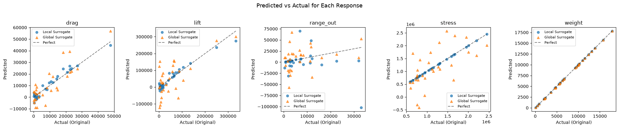
• Visualize with scatter plots (predicted vs actual) and percent error box plots

# --- Generate test sites (distinct from training data) ---
n_test = 30

# Use an optimized Latin Hypercube with a different seed
global_test_sampler = LatinHypercube(d=global_num_vars, optimization='random-cd', seed=999)
global_test_unit = global_test_sampler.random(n=n_test)
global_test_scaled = scale(global_test_unit, global_lower, global_upper)

test_data = {}
for i, var in enumerate(original_evaluator.opt_problem.variables):
    test_data[var.name] = global_test_scaled[:, i]

# Create separate DataFrames for each evaluator (they modify in place)
test_sites_original = pd.DataFrame(test_data).copy()
test_sites_modified = pd.DataFrame(test_data).copy()
test_sites_global = pd.DataFrame(test_data).copy()

# --- Evaluate all three ---
# 1. Original assembly (ground truth)
original_evaluator(test_sites_original)

# 2. Locally-replaced assembly
modified_evaluator(test_sites_modified)

# 3. Global surrogate (PolynomialModel, call directly with DataFrame)
global_surrogate(test_sites_global)

print(f"Test sites: {n_test} points (seed=999)")
print(f"Responses being compared: {original_evaluator.outputs}")

Test sites: 30 points (seed=999)
Responses being compared: ['drag', 'lift', 'range_out', 'stress', 'weight']

# --- Compute error metrics ---
# Using original as baseline truth
error_records = []

for response in original_evaluator.outputs:
    actual = test_sites_original[response].values

    # Local surrogate-replaced assembly errors
    if response in test_sites_modified.columns:
        pred_local = test_sites_modified[response].values
        abs_err_local = np.abs(pred_local - actual)
        rel_err_local = np.abs((pred_local - actual)/actual)
        error_records.append({
            'Response': response,
            'Evaluator': 'Local Surrogate',
            'Mean Absolute Error': abs_err_local.mean(),
            'Max Absolute Error': abs_err_local.max(),
            'Mean Relative Error': rel_err_local.mean(),
            'Max Relative Error': rel_err_local.max(),
        })

    # Global surrogate errors
    if response in test_sites_global.columns:
        pred_global = test_sites_global[response].values
        abs_err_global = np.abs(pred_global - actual)
        rel_err_global = np.abs((pred_global - actual)/actual)
        error_records.append({
            'Response': response,
            'Evaluator': 'Global Surrogate',
            'Mean Absolute Error': abs_err_global.mean(),
            'Max Absolute Error': abs_err_global.max(),
            'Mean Relative Error': rel_err_global.mean(),
            'Max Relative Error': rel_err_global.max(),
        })

error_df = pd.DataFrame(error_records)

# Display summary table
print("Error Summary (relative to original assembly):")
print("=" * 70)
error_df

Error Summary (relative to original assembly):
======================================================================

	Response	Evaluator	Mean Absolute Error	Max Absolute Error	Mean Relative Error	Max Relative Error
0	drag	Local Surrogate	2307.666895	6.065311e+03	2.266751e+00	2.429589e+01
1	drag	Global Surrogate	6010.438387	2.016210e+04	3.866303e+00	2.944095e+01
2	lift	Local Surrogate	13700.275698	5.932725e+04	2.068309e+00	2.418914e+01
3	lift	Global Surrogate	57068.666622	1.503073e+05	1.078248e+01	1.424657e+02
4	range_out	Local Surrogate	14259.976964	1.354810e+05	2.933932e+00	3.406858e+01
5	range_out	Global Surrogate	19629.343607	6.400622e+04	6.532330e+00	2.706684e+01
6	stress	Local Surrogate	0.000000	0.000000e+00	0.000000e+00	0.000000e+00
7	stress	Global Surrogate	437748.209473	1.218308e+06	4.173909e-01	1.593590e+00
8	weight	Local Surrogate	0.000000	0.000000e+00	0.000000e+00	0.000000e+00
9	weight	Global Surrogate	0.000021	6.932602e-05	1.266153e-08	2.577760e-07

# --- Scatter plots: predicted vs actual for each response ---
n_responses = len(original_evaluator.outputs)
fig, axes = plt.subplots(1, n_responses, figsize=(4 * n_responses, 4))

if n_responses == 1:
    axes = [axes]

for idx, response in enumerate(original_evaluator.outputs):
    ax = axes[idx]
    actual = test_sites_original[response].values

    # Plot local surrogate predictions
    if response in test_sites_modified.columns:
        ax.scatter(actual, test_sites_modified[response].values,
                   alpha=0.7, label='Local Surrogate', marker='o', s=30)

    # Plot global surrogate predictions
    if response in test_sites_global.columns:
        ax.scatter(actual, test_sites_global[response].values,
                   alpha=0.7, label='Global Surrogate', marker='^', s=30)

    # Perfect prediction line
    lims = [min(actual.min(), actual.min()), max(actual.max(), actual.max())]
    ax.plot(lims, lims, 'k--', alpha=0.5, label='Perfect')

    ax.set_xlabel('Actual (Original)')
    ax.set_ylabel('Predicted')
    ax.set_title(response)
    ax.legend(fontsize=8)

plt.suptitle('Predicted vs Actual for Each Response', fontsize=13, y=1.02)
plt.tight_layout()
plt.show()

# --- Percent error box plots grouped by evaluator ---
fig, axes = plt.subplots(1, n_responses, figsize=(4 * n_responses, 4))

if n_responses == 1:
    axes = [axes]

for idx, response in enumerate(original_evaluator.outputs):
    ax = axes[idx]
    actual = test_sites_original[response].values

    # Compute percent errors (avoid division by zero)
    pct_errors = {}
    mask = np.abs(actual) > 1e-10  # Only compute where actual is non-zero

    if response in test_sites_modified.columns:
        pred_local = test_sites_modified[response].values
        pct_err_local = np.where(mask, (pred_local - actual) / actual * 100, 0.0)
        pct_errors['Local\nSurrogate'] = pct_err_local

    if response in test_sites_global.columns:
        pred_global = test_sites_global[response].values
        pct_err_global = np.where(mask, (pred_global - actual) / actual * 100, 0.0)
        pct_errors['Global\nSurrogate'] = pct_err_global

    if pct_errors:
        ax.boxplot(pct_errors.values(), tick_labels=pct_errors.keys())

    ax.axhline(y=0, color='k', linestyle='--', alpha=0.3)
    ax.set_ylabel('Percent Error (%)')
    ax.set_title(response)

plt.suptitle('Percent Error by Evaluator for Each Response', fontsize=13, y=1.02)
plt.tight_layout()
plt.show()

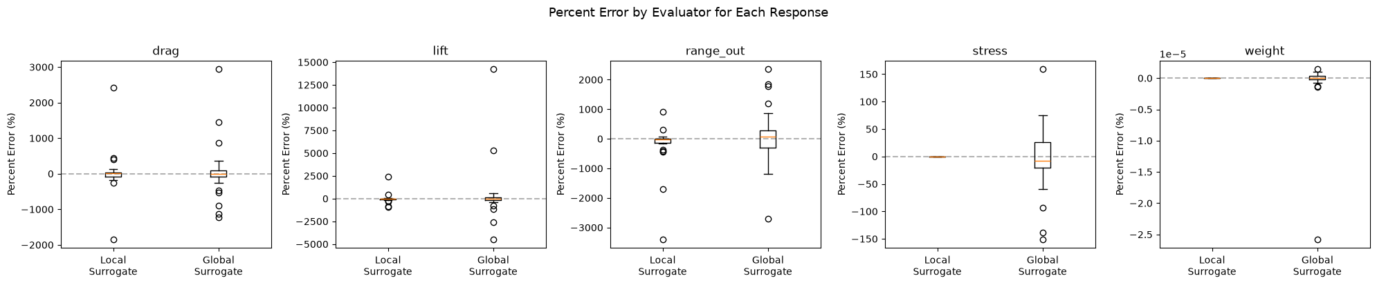
Looking at the results we see that the local model of course is perfect for stress and weight since those are not approximated by a surrogate model. The results for the responses from the aero component are not as clear.